Data preparation
The data in machine learning is presented in the form of a matrix (data frame in R) consisting of N rows (samples or instances) and M columns (features).
Features
Features can be different types:
- Binominal (TRUE/FALSE)
- Categorial/nominal (different classes)
- Text - not supported by all applications
- Numeric (Real numbers)
- Integer (Natural numbers)
Note that a common mistake is to mischaracterize features. Nominal values are usually presented by numbers but cannot be compared. If not set properly, errors could occur.
Example: Many choose to set education status as 1: no college, 2: college degree, 3: post-graduate. Ask yourself, does 1.5 have a meaning?
Example: Stages of a tumor is represented by numbers (1, 2, ..) but it nominal.
Special features include the ID, label, batch, etc. They are treated differently. ID is excluded from models and must be unique. Label is used for supervised learning (classification). A dataset can only have one label (per each run).
Meta-features are features made using the measured features. For example BMI is a feature made from weight and height. PCA vectors are features based on all features.
Data exploration
Explore the data to validate your data and potentially find new patterns. Data validation means that you should show known relations shown in the literature is present in your data. For example if a gene has been highly associated with your case studies, you should observe the same pattern in your data. Or if you have blood pressure and heart disease, they should be correlated. In addition you should show your data is representative of the real population. For example if you are working on samples from USA and you have an obesity feature (not label) you should make sure that the ratio of obese people is comparable to the ratio in USA. Or if the ratio of female to male is about 50%.
Draw many plots. Show how the features are distributed and how you expect them to be. Show your data is balanced (e.g. female and male have the same ratio) and if not be aware of the imbalance (for example rare diseases). The probability distributions in your data can result in misinterpretation.
In order to validate your data you can look for correlations between numeric features and associations between nominal features. The known relations in the literature should be validated by your data. You might find new relations and associations which can further be studied.
Let’s look at an example on as subset of features patients with diabetes type 2.
     age       sex      education   living     smoking      weight           height           LDL             HDL
Min.   : 4.0   F:1688   1   :976   1   :1319   0:2148   Min.   : 16.00   Min.   : 83.0   Min.   : 11.0   Min.   : 16.0
1st Qu.:45.0   M: 757   2   :753   2   : 872   1: 130   1st Qu.: 61.00   1st Qu.:151.0   1st Qu.: 56.0   1st Qu.: 45.0
Median :52.0            3   :377   NA's: 254   2:  23   Median : 71.00   Median :157.0   Median :106.0   Median : 60.0
Mean   :51.6            NA's:339               3: 144   Mean   : 73.73   Mean   :157.9   Mean   :104.3   Mean   :106.8
3rd Qu.:60.0                                            3rd Qu.: 87.00   3rd Qu.:165.0   3rd Qu.:141.0   3rd Qu.:160.0
Max.   :89.0                                            Max.   :161.00   Max.   :196.0   Max.   :700.0   Max.   :665.0
NA's   :15                                              NA's   :332      NA's   :620     NA's   :587     NA's   :404
Education is the level of education (1=finished high school, 2=college degree, 3=post graduate) and living is the type of living environment (1=city/town, 2=village). Smoking is another nominal feature (0=doesn’t smoke, 1: occasional smoker, 2=light smoker, 3=heavy smoker). HDL and LDL are good and bad cholesterol levels in blood. Missing data is represented with NAs.
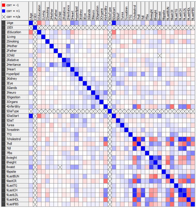
1. Correlation matrix: calculate the correlation between the features and draw a heatmap. Look at the highly correlated features. Make sure the correlations are valid (by literature) and mark down if they are direct correlations or indirect.
2. Association rules: find associations between sets of features to another feature. Each rule associates a set of features to another feature. The rule certainty is measured using two parameters: support or frequency (how much of the data supports it) and confidence (out of all applicable data points, how many follow the rule). Association rules are applied on nominal features or discrete values.
> library(arules)
> rules <- apriori(data, parameter=list(support=0.10, confidence=0.50))
Apriori

Parameter specification:
 confidence minval smax arem  aval originalSupport maxtime support minlen maxlen target   ext
        0.5    0.1    1 none FALSE            TRUE       5     0.1      1     10  rules FALSE

Algorithmic control:
 filter tree heap memopt load sort verbose
    0.1 TRUE TRUE  FALSE TRUE    2    TRUE

Absolute minimum support count: 244

set item appearances ...[0 item(s)] done [0.00s].
set transactions ...[26 item(s), 2445 transaction(s)] done [0.00s].
sorting and recoding items ... [23 item(s)] done [0.00s].
creating transaction tree ... done [0.00s].
checking subsets of size 1 2 3 4 5 done [0.00s].
writing ... [477 rule(s)] done [0.00s].
creating S4 object  ... done [0.00s].
> rules
set of 477 rules
    > inspect(head(rules, n = 10, by ="lift"))
     lhs                                             rhs                support   confidence lift     count
[1]  {sex=M,smoking=0,weight=[80,161]}            => {height=[162,196]} 0.1132924 0.7527174  2.997384 277
[2]  {sex=M,weight=[80,161]}                      => {height=[162,196]} 0.1525562 0.7474950  2.976588 373
[3]  {sex=M,smoking=0,height=[162,196]}           => {weight=[80,161]}  0.1132924 0.8683386  2.920341 277
[4]  {sex=M,height=[162,196]}                     => {weight=[80,161]}  0.1525562 0.8477273  2.851022 373
[5]  {weight=[80,161],height=[162,196]}           => {sex=M}            0.1525562 0.8555046  2.763156 373
[6]  {smoking=0,weight=[80,161],height=[162,196]} => {sex=M}            0.1132924 0.8195266  2.646952 277
[7]  {height=[162,196]}                           => {weight=[80,161]}  0.1783231 0.7100977  2.388155 436
[8]  {weight=[80,161]}                            => {height=[162,196]} 0.1783231 0.5997249  2.388155 436
[9]  {sex=M,smoking=0}                            => {height=[162,196]} 0.1304703 0.5885609  2.343699 319
[10] {smoking=0,height=[162,196]}                 => {weight=[80,161]}  0.1382413 0.6954733  2.338971 338
You should make sure that all the top rules are meaningful. For example: {age=[57,89]} => {education=1} makes sense since the data was collected in a medium size city in the south of Iran, and the older people were most likely uneducated.
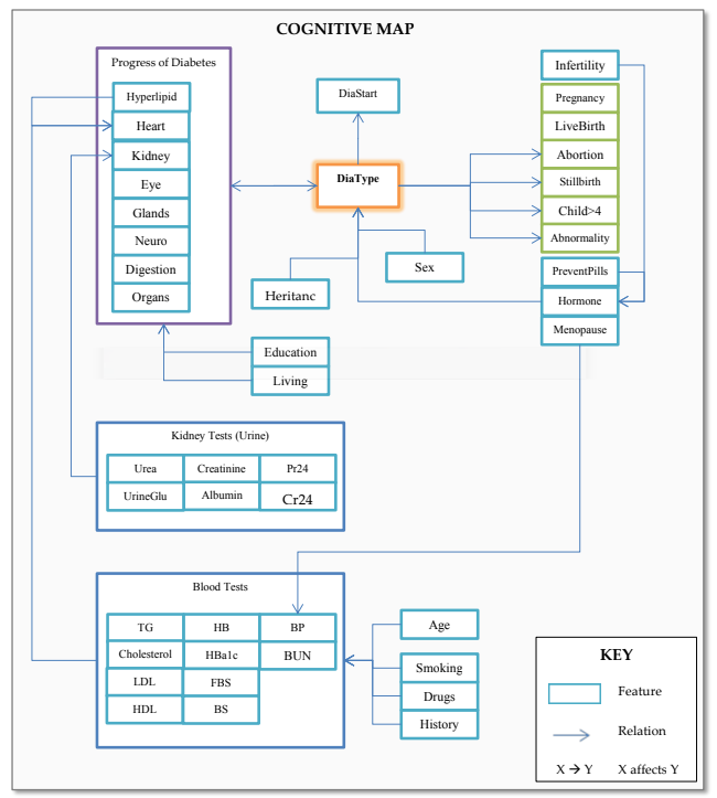
3. Cognitive map shows the relations known in your data and the ones you also found.
Data preparation
The most important but neglected part of machine learning and data mining is preparing the data. If your data is invalid, no matter what skills you have, the results will be invalid. The goal of data preparation is to make sure the data is representative and correct.
1. Typos are the most common error in data. Most datasets are collected over time, manually input by operators. For any nominal value you should check the levels in the data. For example for sex make sure you only have 2 levels (F/M or female/male). For numeric values draw boxplots and histograms. Make sure the data follows the expected distribution and estimates (mean and standard deviation are same as expected). If you have nominal features, make sure the numeric values for each are correctly spread out. For example if you have sex and age in your data, make sure the age distribution for female and male are comparable.
2. Missing data is common. Make sure they are presented in a correct format recognized by the tool and code you use. Some tools take NA or blanks as missing, some use “?”. Make a table and see which data points are missing and how often. Try to understand why and if it is randomly missing or has a pattern? Decide how to handle them. Some methods accept missing values and some don’t. Understand how missing values are interpreted. If you remove them have a good explanation of your criteria. Some might choose to replace missing data with nearby datapoints if possible.
3. Normalization is an important step to make the samples and features comparable inside and in between datasets. Choose an appropriate normalization method and explain how it was done. In case of classification, the test has to be normalized in the same way but independent of the train data to avoid leaking train information into test.
Expression data is usually log2 transformed and then quantile normalized. RMA and frozen-RMA are versions of quantile normalization common for microarray datasets which handle outliers better. zscore is a intuitive normalization method but flattens the data (forces them into a normal) and range normalization keeps the distribution but is very sensitive to outliers. Centering numeric values around zero is a good practice for some models. It is a good practice to make features in the same range to be able to compare the weights assigned to each fature by a model. For example if you have a feature in the order of thousands and a feature in the order of 10, the weights might seem smaller for the former, while the truth is the weights cannot be directly compared. Note than normalizing can be applied on features (normalizing measurements over all samples) or on samples (correcting for batch effects).
4. Feature selection and reduction is used to chose relevant features. Note that the number of features should be significantly less than the sample size (M<<N). In general a model with less parameters is a better model and is less likely to overfit. Redundant features (usually very highly correlated features) should be removed for some models (any model doing determinant on the data matrix). Principle Component Analysis is a good practice to reduce the number of features while maintaining the variability. Feature selection can be done based on variability (keeping highly variable features), fold changes (difference in mean between label classes such as deferentially expressed genes in gene expression data), or recursively by applying a classification model and applying the weights (choosing the features with highest importance). Feature reduction can be done based on correlation (removing highly correlated features) or invariability (features which have similar distributions between classes). Note that in case of classification feature selection should be done only on the train data and not test.
After data preparation, you should be able to explain the data in terms of what features there are and what distributions they follow. You should show your data is representative and balanced. You should handle missing data in a rational way. You should have a well established method for choosing features.