Supervised learning¶

For supervised learning, we employ learning algorithms which are able to generate estimates of an outcome variable based on a set of predictor variables.

There are two types of supervised learning: regression and classification. For regression the outcome variable is a numeric value, for which learning algorithms try to minimize the error or distance of the predictions of this value and the true value. For classification the outcome variable is a label or category for which learning algorithms try to minimize the rate at which our prediction of this label or category is wrong. Often the same or slightly tweaked versions of a method can be employed to perform either task. Below we list some examples of supervised learning algorithms.

Examples of supervised learning¶

Generalized linear regression¶

Linear regression learns a linear combination of the values of the predictor variables to make unbiased estimates of a numeric outcome variable.
Logistic regression is similar to linear regression but applies to a binary outcome variable. It estimates the log-odds that an outcome variable is of one-of-two labels based on a linear combinations of the values of a predictor variables.

Linear classifiers¶

Support Vector Machine (SVM) learns a hyperplane which separates the values of a binary outcome variable based on a set of predictor variables.
Linear Discrimant Analysis learns multivariate gaussian distribution for each label of a categorical outcome variable based on the set of predictor variables. Predictions are then made based on the relative probability that an new observation came from each distribution.

Probability based¶

These models use probability to predict the label.

Naive-bayes uses Bayes theorem on the feature distribution and probabilities. Usually is used as a baseline model (default or worse).
K nearest neighbors (KNN) predicts each sample based on majority vote of its K nearest neighbors (the K most similar samples).

Tree based¶

Decision trees learn a set of rules for predicting the outcome variable from a set of predictor variables by recursively splitting the data into two-or-more subsets. For each split, it finds a rule for which the outcome variable of the observations that follow that rule are more similar than those that do not. These are handy for both regression and classification tasks.

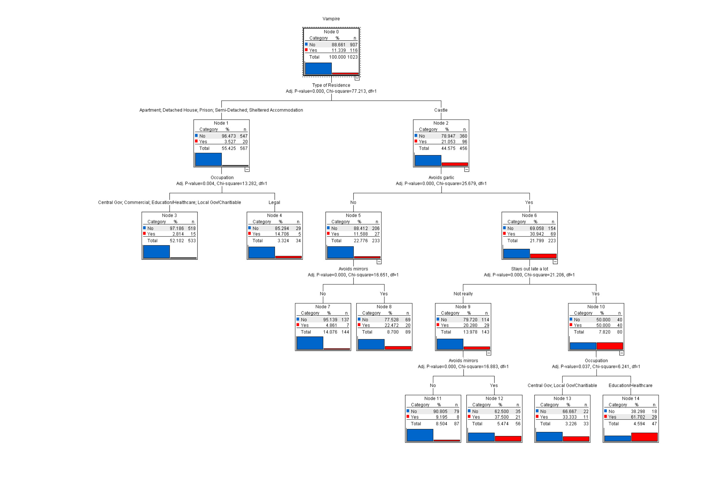
Below is a decision tree to predict if a sample is a vampire. Each branch ask a question and based on that divides the samples. Following the branches you get to a leaf which is labeled by the label majority of the train samples ending there.

Random forest is an algorithm which generates a set of decision trees. For each tree the forest, it perturbs the data using one-or-more sampling methods, in order to create trees that are relatively uncorrelated and will make different predicitons. Random forests is referred to as an ensemble method because the final prediction is based on ensemble of predictions made by each tree.

Assessing model performance¶

A common problem in supervised machine learning is what is called overfitting. Overfitting arises when the error of predicting the values of the outcome variable of the observations used to learn or train the model is very low, but the model is not useful for predicting the values of outcome variables for new observations which were not used for learning the model. For this reason, model performance is commonly assessed by randomly separating an initial data set into a training set, and a test set. The model is learned (or trained) using the training data and then the error is estimated using the test data. A critical part in supervised learning is to make sure the train data does not leak into the test, meaning no data in the train set should be present also in the test set - whether at normalization, feature selection, or when learning the model.

If enough data is available, it is common to randomly split the data into three subsets. Here, a validation data set is used to tune the parameters of the model generated by the training data.

Cross validation¶

Cross validation is a method employed for assessing model performance and model tuning. In either case, the main advantage of cross validation is it greatly reduces the amount of data necessary for training and testing a model.

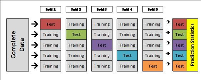
An illustration of cross validation is shown below. Here we divide the data into K subsets of equal or near equal size. For example in 10-fold crossvalidation, we divide the data into ten subsets. We then train 10 different models, each model is trained using 90% and then the model is tested on the remaining 10%. The final performance will be based on the testing error across all 10 models.

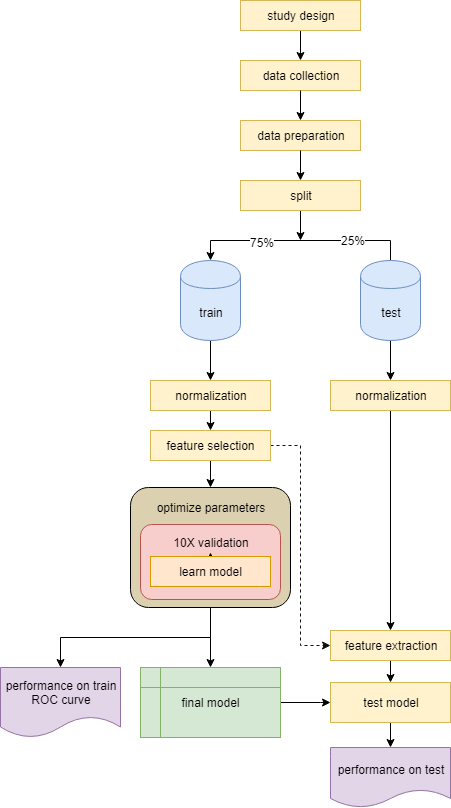
A workflow that incorporates cross-validation in model training is shown below …

Performance of a regression model¶

Assessing the performance of a regression model is fairly straight forward. We have to measure the error of the prediction, e.g. how close to the real values are the predicted values. Two fitness measures for regression are:

Mean Squared Error (MSE)

\[MSE = \frac{1}{N} \sum{(label_{predicted} - label_{actual})^2}\]

Root Mean Squared Deviation (RMSD)

\[RMSD = \sqrt{\frac{\sum{(label_{predicted} - label_{actual})^2}}{N}}\]

Performance of a classification model¶

On the other hand, assessing the performance of a classification model is more nuanced. There are many different performance metrics and the level to which one regards one compared to another is specific to the task at hand.

Confusion matrix is a table showing how the samples were classified. The columns show the actual labels and the rows are the predicted labels.

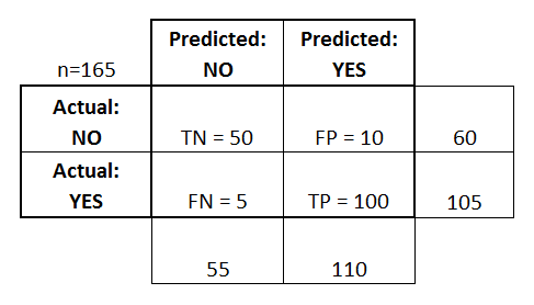
TN=true negative (samples predicted to be in class negative and that was correct)
TP=true positive (samples predicted to be in class positive and that was correct)
FN=true negative (samples predicted to be in class negative and that was incorrect)
FP=true positive (samples predicted to be in class positive and that was incorrect)

If you show the performance of the model as a confusion matrix, fitness can be measured by 4 main criteria:

Accuracy

\[\frac{TP + TN}{TP + FP + TN + FN}\]

Sensitivity

\[\frac{TP}{TP + FN}\]

Precision

\[\frac{TP}{TP + FP}\]

Specificity

\[\frac{TN}{TN + FP}\]

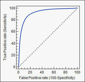
Receiver operating characteristic (ROC) curve illustrates the performance of a model based on different decision boundaries when making binary predictions. For each decision boundary we calculate the sensitivity and specificity and plot the resulting curve. The area under the curve (AUC) is simply the error under this curve. If there exists a decision boundary for which the sensitivity and specificity are both perfect, i.e. 1, then the AUC will be 1. In contrast, poorly fit models will have AUC close to 0.5.